Run ANUGA Yourself
Everything Hydrata computes on cloud compute, you can also compute on your own machine. The same simulation engine ships as a single standalone executable for Windows and Linux: no Python, no installers, no dependencies. Point it at a scenario package and it runs the same ANUGA solver and the same pipeline, producing directly comparable results.
This is useful for:
- Verifying a Hydrata result independently on your own hardware
- Working offline, or inside networks where cloud access is restricted
- Inspecting exactly what a Scenario contains before or after a Run
1. Get your scenario package
A scenario package is a self-contained folder: a scenario.json configuration plus an inputs/ folder of terrain and forcing data. It is everything the solver needs. See Package Format for the directory layout and scenario.json Reference for every configuration field.
You can get one two ways:
Download from Hydrata
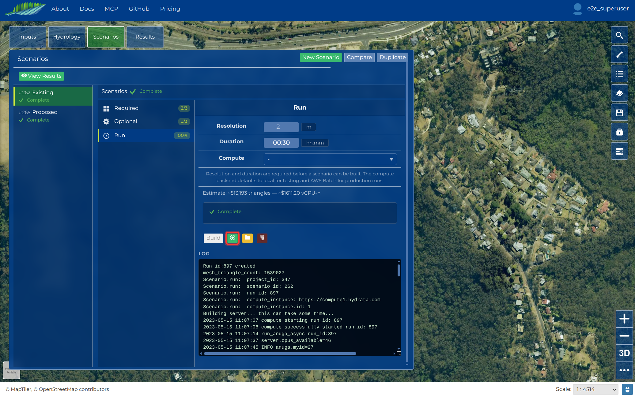
- Open your project and go to the Scenarios panel
- Build the Scenario you want (click Build); its status changes to Built when the package is ready
- Click the download button on the Scenario to save the scenario package as a zip
- Extract the zip somewhere convenient
Note
Building a Scenario is what produces the scenario package. A Scenario that has never been built has nothing to download yet.
Or use the bundled example
The executable download (next step) includes a small worked example at examples/small_test/: a 200 m x 200 m domain with a 1 m DEM, uniform rainfall, and a 30 minute duration. It runs in a few minutes on a laptop, so it is the quickest way to confirm everything works before you bring your own data.
2. Download the executable
Download the build for your platform from the latest release:
| Platform | Download | Notes |
|---|---|---|
| Ubuntu 22.04 | run-anuga-ubuntu2204.tar.gz |
glibc 2.35, broadest Linux compatibility |
| Ubuntu 24.04 | run-anuga-ubuntu2404.tar.gz |
glibc 2.39 |
| Windows | run-anuga-windows.zip |
Windows SmartScreen
On first launch Windows will likely show a "Windows protected your PC" warning. Click More info, then Run anyway. This is normal for unsigned executables.
After extracting you'll have:
run-anuga              # (run-anuga.exe on Windows)
examples/
  small_test/
    scenario.json
    inputs/
      dem.tif
      boundary.geojson
      inflow.geojson
3. Validate, inspect, run, post-process
Open a terminal (Linux) or Command Prompt / PowerShell (Windows) and cd into the extracted folder. The commands below use the bundled example; substitute the path to the scenario.json (or its folder) inside the scenario package you downloaded from Hydrata to simulate your own model instead.
Platform syntax
Examples are shown for both platforms. On Windows use .\run-anuga.exe and backslashes in paths. PowerShell requires the .\ prefix; Command Prompt works with or without it.
Validate the package
Checks the scenario.json and inputs before committing to a simulation:
Expected output:
Inspect the configuration
Prints a summary of the package: inputs, parameters, and coordinate system.
Run the simulation
The example takes roughly 1-3 minutes. Progress is logged as percentage complete with elapsed time. When it finishes, results appear in an outputs folder next to the package contents (for the example, examples/small_test/outputs_1_1_1/). Runtime for your own packages scales with domain size, mesh resolution, and duration.
Post-process to GeoTIFF
The run command post-processes automatically, so you normally don't need this step. Use it to regenerate the GeoTIFF rasters from an existing .sww result, for example at a different raster resolution:
4. Outputs
Post-processing turns the solver's native time-series into standard GeoTIFF rasters:
outputs_1_1_1/
  run_1_1_1.sww                                  Full time-series (NetCDF)
  run_1_1_1_depth_max.tif                        Max water depth
  run_1_1_1_velocity_max.tif                     Max flow velocity
  run_1_1_1_depthIntegratedVelocity_max.tif      Max depth x velocity
  run_1_1_1_stage_max.tif                        Max water surface elevation
  run_1_1_1_depth_000060.tif                     Depth at t=60s (one per timestep)
  ...
  run_anuga_1.log                                Simulation log
  checkpoints/                                   Restart files
The *_max.tif files are the main outputs for design work: the peak value of each quantity at every cell across the whole simulation. The per-timestep rasters let you step through the event in time. All of them load directly into QGIS, ArcGIS, or any GIS software (nodata value is -9999).
The full GeoTIFF set, including the stage rasters, is always available to download from a Run. Online, however, Hydrata publishes only Depth Max, Velocity Max, and Momentum (depth-integrated velocity) Max as default map layers; stage is computed and downloadable but is not surfaced as a map layer on the platform.
| Quantity | Units | Description |
|---|---|---|
depth |
m | Water depth above ground surface |
velocity |
m/s | Flow speed |
depthIntegratedVelocity |
m²/s | Depth x velocity, relevant for flood hazard assessment |
stage |
m | Water surface elevation (ground + depth) |
These are the same rasters Hydrata produces when a Run completes on cloud compute: the platform runs this same pipeline, then publishes the Depth, Velocity, and Momentum maxima as map layers you can explore in the browser. So a local result and an online Run of the same built Scenario are directly comparable. See Viewing Results for how Hydrata presents them online.
5. Advanced: install as a Python package
If you want to modify the code, embed simulations in your own pipelines, or run large jobs in parallel on a Linux cluster, install run_anuga from source instead of using the executable. This route also suits HPC and batch environments: ANUGA supports MPI domain decomposition on Linux, so big domains can be split across many cores, and the CLI is easy to script for parameter sweeps or CI.
# 1. Clone the repo
git clone https://github.com/Hydrata/run_anuga.git
cd run_anuga

# 2. Install system dependencies (Ubuntu/Debian)
sudo apt-get install build-essential gfortran \
    libopenmpi-dev openmpi-bin \
    libhdf5-dev libnetcdf-dev

# 3. Install run_anuga with simulation dependencies
pip install -e ".[sim,dev]"

# 4. Install ANUGA and its undeclared runtime dependencies
pip install anuga mpi4py matplotlib scipy triangle netCDF4 pymetis

# 5. Run the test scenario
run-anuga validate examples/small_test/scenario.json
run-anuga run examples/small_test/scenario.json
All Python dependencies install from binary wheels, so no system-level GDAL, PROJ, or GEOS is needed. The anuga package (v3.2) only declares numpy in its metadata but needs the extra packages in step 4 at import time.
The package defines several extras: [sim] for simulation dependencies (rasterio, numpy, shapely, geopandas), [viz] for visualisation, [platform] for Hydrata platform integration, [dev] for test tooling, and [full] for everything. Bare pip install run_anuga gives just config parsing, validation, and the CLI.
The Python API mirrors the CLI:
from run_anuga.run import run_sim
from run_anuga.callbacks import LoggingCallback

run_sim("/path/to/package", callback=LoggingCallback())
Modifying ANUGA itself
If you need to change the solver rather than the runner, clone anuga_core separately and pip install -e . from that directory instead of the PyPI package.
Next steps
- Package Format: what's inside a scenario package
- scenario.json Reference: every configuration field
- Defaults: the simulation constants the runner applies
- Concepts: how ANUGA's solver works