Viewing Results
When a Run reaches Complete, Hydrata publishes its outputs back to your project. This page explains how you get to them, what each one shows, how to read a profile along a line you draw, and how to compare two Scenarios.
The moving picture of a Run has its own page: see Playing Back a Run.
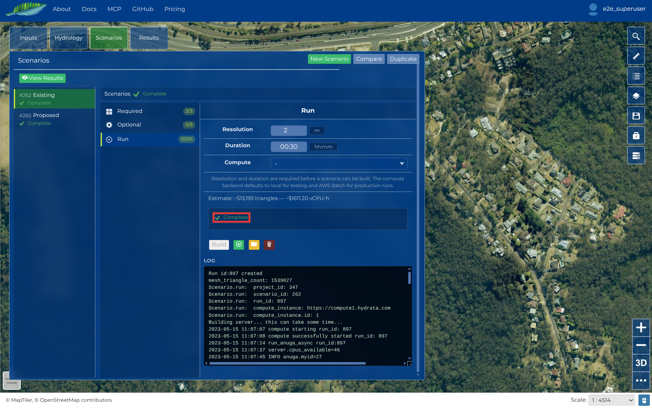
Watching a Run finish
Select your Scenario in the Scenarios panel and open its Run tab. The status pill steps through the Run lifecycle:
Created > Building... > Built > Queued > Computing > Processing results... > Complete
A Scenario rests at Built until you dispatch the Run, unless you used the combined Build and Run action. While the Run is Computing, the status card shows a progress percentage and an estimated time remaining. Processing results... means the simulation itself has finished and Hydrata is turning the outputs into layers and the playback store. If something goes wrong the pill shows Error with a plain-English failure message, and a Retry button appears.
Getting to the results
Open the Results menu, either with the View Results button that appears on a completed Scenario in the Scenarios panel, or with Results in the left toolbar.
The Results menu is a list of Scenarios, one row each, not a list of layers. Clicking a row loads that Scenario's most recent completed Run in the player and starts it. The Cross-section button lives in the same menu.
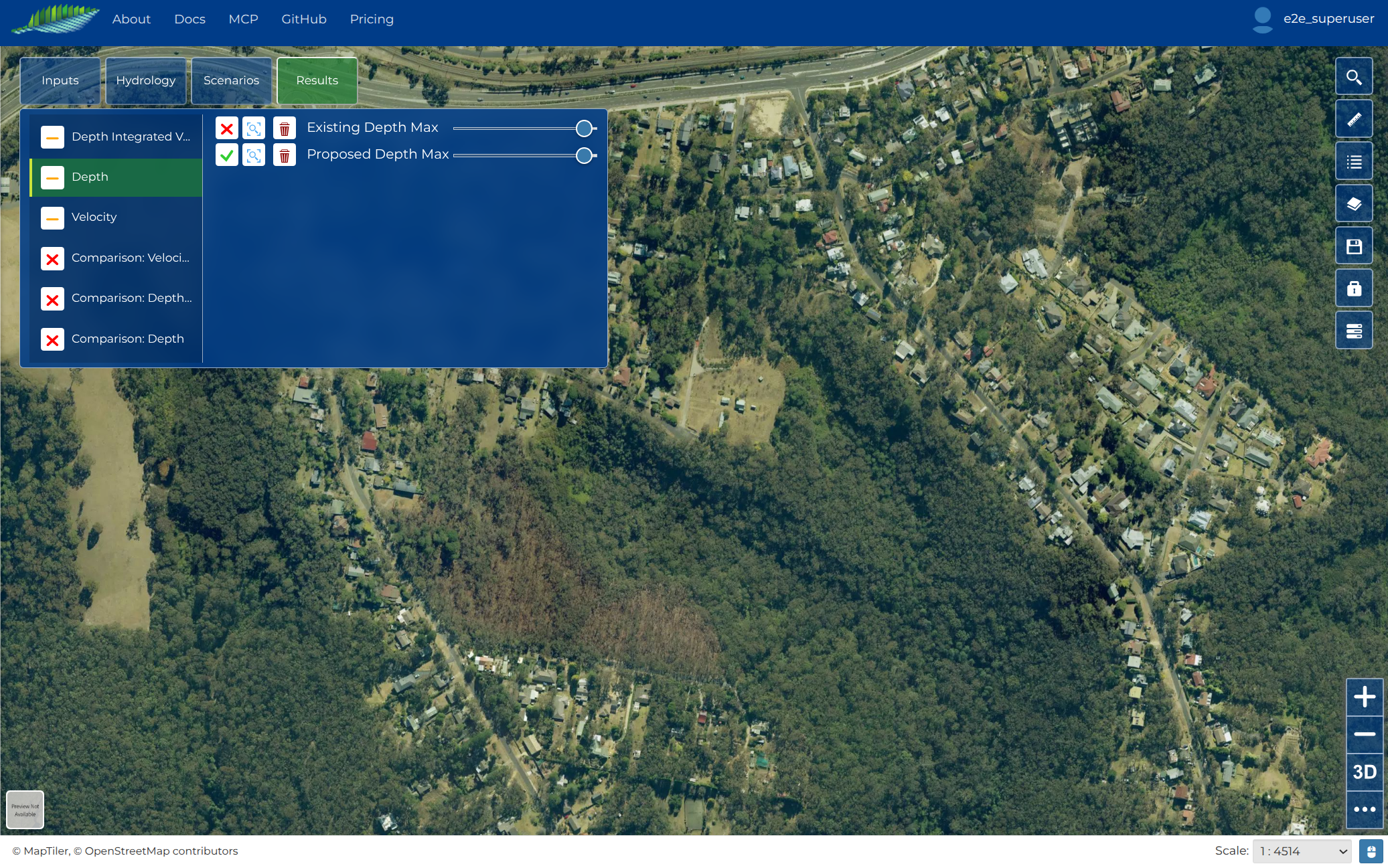
Nothing result-shaped paints when a map opens
Opening a project never drops a flood on top of your inputs, however many Runs the project has. Result layers arrive hidden, deliberately, so that a map with eight Runs on it opens showing your terrain and your inputs. The peak view is something you ask for, with Max in the player.
If the Scenario has been run more than once, a banner tells you when the results on screen are not from the newest Run: it names the Run you are looking at, and says whether the newer one failed or is still building.
The maximum-value layers
Each completed Run publishes three rasters as datasets in your catalogue, named after the Scenario. They are not drawn on the project map, and the map has no layer list to switch them on from: the peak view inside the app is the player's Max control, and a raster on its own is reached from its dataset page in the catalogue or from the download.
| Layer | Group | What it shows | Units |
|---|---|---|---|
| Scenario name Depth Max | Depth | Maximum water depth reached at each point | metres |
| Scenario name Velocity Max | Velocity | Maximum flow speed reached at each point | m/s |
| Scenario name Momentum Max | Momentum | Maximum depth-integrated velocity (depth multiplied by velocity), a common flood-hazard indicator | m²/s |
Each layer is named after the Scenario that produced it, so results from different Scenarios in the same project stay distinguishable. They are the same GeoTIFFs you get from the download, rendered by the server, which makes them the right thing to take into your own GIS and the wrong thing to read a single moment from.
These are maximum envelopes, not snapshots
Each cell shows the highest value it reached at any time during the simulation. Different cells can peak at different times, so a maximum layer is not a picture of one moment in the flood. It answers "how bad did it get here", which is usually the question that matters for planning and design. For one moment, use playback.
See ANUGA Concepts for the physical definitions of depth, velocity, stage, and momentum.
Maximum layers vs the full time series
The full time history is preserved as well. ANUGA writes the complete time series to an SWW file, Hydrata generates one GeoTIFF per output timestep for each quantity (including stage, the water surface elevation), and the playback store holds the depth and velocity fields on the mesh. The per-timestep GeoTIFFs and the SWW are not published as map layers; they are in the downloadable result files. See Exporting Results.
Reading the map
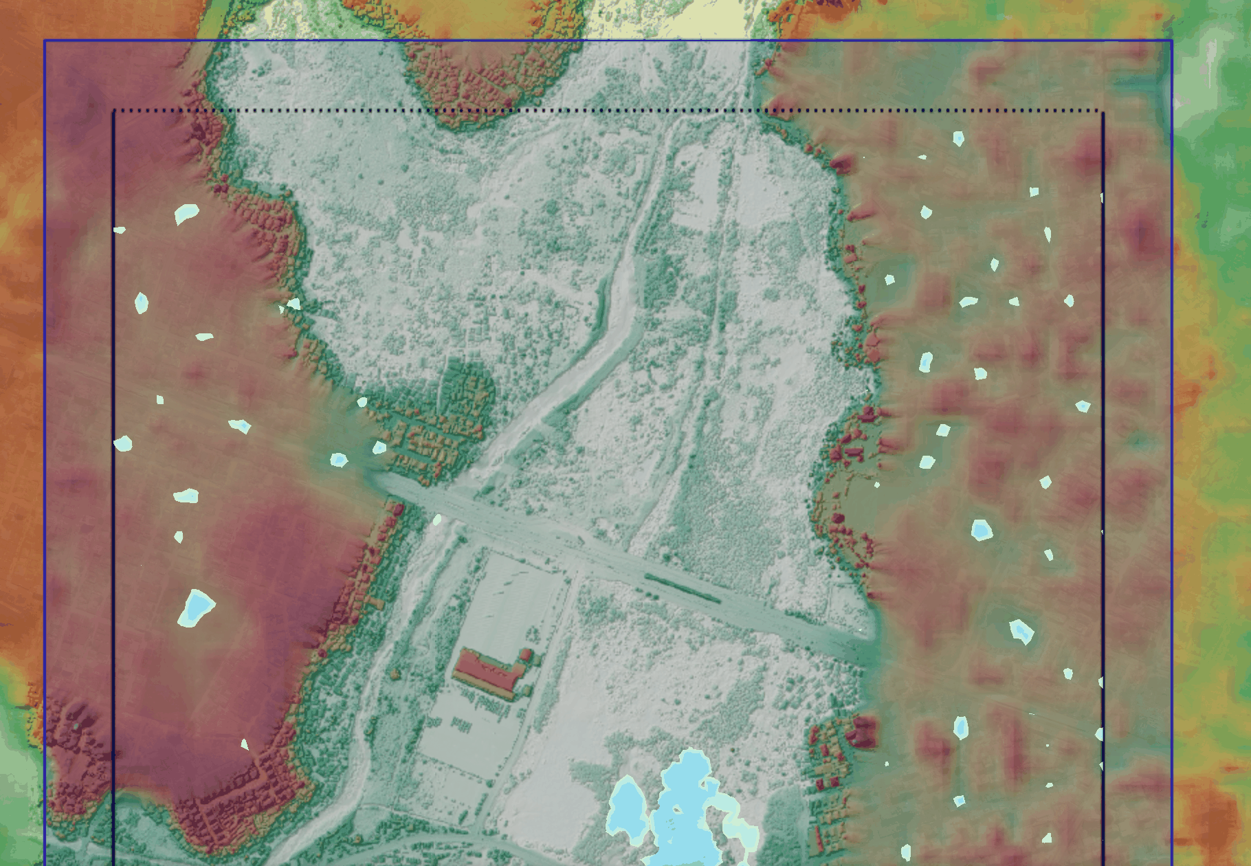
- Dry ground is transparent. Cells the water never reached have no value, so the terrain and basemap show through.
- Very shallow water is hidden. The depth style is fully transparent below 0.05 m and fades in from 0.10 m, so films of water a few centimetres deep do not clutter the map.
- Default colour ramps: depth shades from pale blue-green to dark blue across 0 to 6 m; velocity runs 0 to 6 m/s; momentum runs 0 to 5 m²/s. The dataset page's legend shows the ramp.
Opacity
The player's Display drawer holds the result opacity, the background opacity and the colour scale for playback. A raster opened from its dataset page has the ordinary dataset viewer's transparency control.
Cross-section along a line you draw
The Cross-section tool answers the question a map cannot: what the ground and the water surface look like along a line. Open it with the Cross-section button in the Results menu.
- Tick what you want on the chart. Rows are grouped into Terrain and Water surface, with up to three of each. The water-surface rows are your Scenarios; one that has nothing to sample yet says why instead of letting you tick it.
- Click Draw profile line, then click points along the map and double-click to finish.
- Read the chart: distance along the line on the x axis, elevation in metres on the y axis. Terrain traces and water-surface traces use separate palettes, and the row list is the legend.
The panel drags by its header and resizes from its corner, and it remembers where you put it. The chart has zoom and reset controls. Clear removes the line so you can draw another.
What the hints on the rows mean:
| Hint | Meaning |
|---|---|
| No terrain is ready | Add or load a terrain before drawing a profile |
| No completed run yet | That Scenario has nothing to sample a water surface from |
| Re-run to get a water surface | The Run predates the stage output the water surface needs |
| Results may be stale | The Scenario was edited after this Run finished |
| Terrain replaced | A newer terrain superseded this one, so draw a new line |
| Uncheck another row first | Three rows per group is the limit |
The chart is for reading on screen. To take the numbers away, export the result rasters and sample them in your own tools: see Exporting Results.
Comparing two Scenarios
The most common results question is "what changed": existing versus proposed conditions, before versus after a mitigation work, one rainfall event versus another. Both Scenarios need a completed Run. There are three ways to read the difference today, and the cross-section is the most direct.
Overlay their water surfaces on one cross-section. Tick two Scenarios in the Water surface group, draw a line through the area you care about, and read the two profiles against the same terrain. This is the quickest defensible comparison because it puts numbers on one chart at the same stations.
Play them one after the other. Load one Scenario in the player, watch the flood develop, then load the other from the Results menu. Loading a run resets the player to its defaults, and those defaults are the same for every run, so two runs do open on the same colour scale. The catch is the other way round: any ceiling, floor, quantity or overlay you changed for the first run is gone when the second one loads, so set them again before you read anything off the colours.
Difference the rasters in your own GIS. Download both Runs' maximum GeoTIFFs and subtract them, or connect your GIS to the layers over OGC services. See Exporting Results. This is the route to take when you need a difference map as a deliverable.
Keep the scale fixed
Whichever route you take, compare like with like: the same quantity, the same colour scale ceiling and the same cross-section line. A change in the scale can look exactly like a change in the flood.
Related pages
- Playing Back a Run for the player, its controls and what a visitor to a public project sees
- Exporting Results for downloads, OGC services and the scenario package
- Troubleshooting if a Run failed, or its results are not where you expect them